Graph neural networks (GNN)

In Machine Learning, neural networks are built from functional building blocks such as dense layers, attention mechanisms, convolution layers and so on.

In this article, we describe the building blocks of graph neural networks (GNNs).

Message passing layer[1][2]

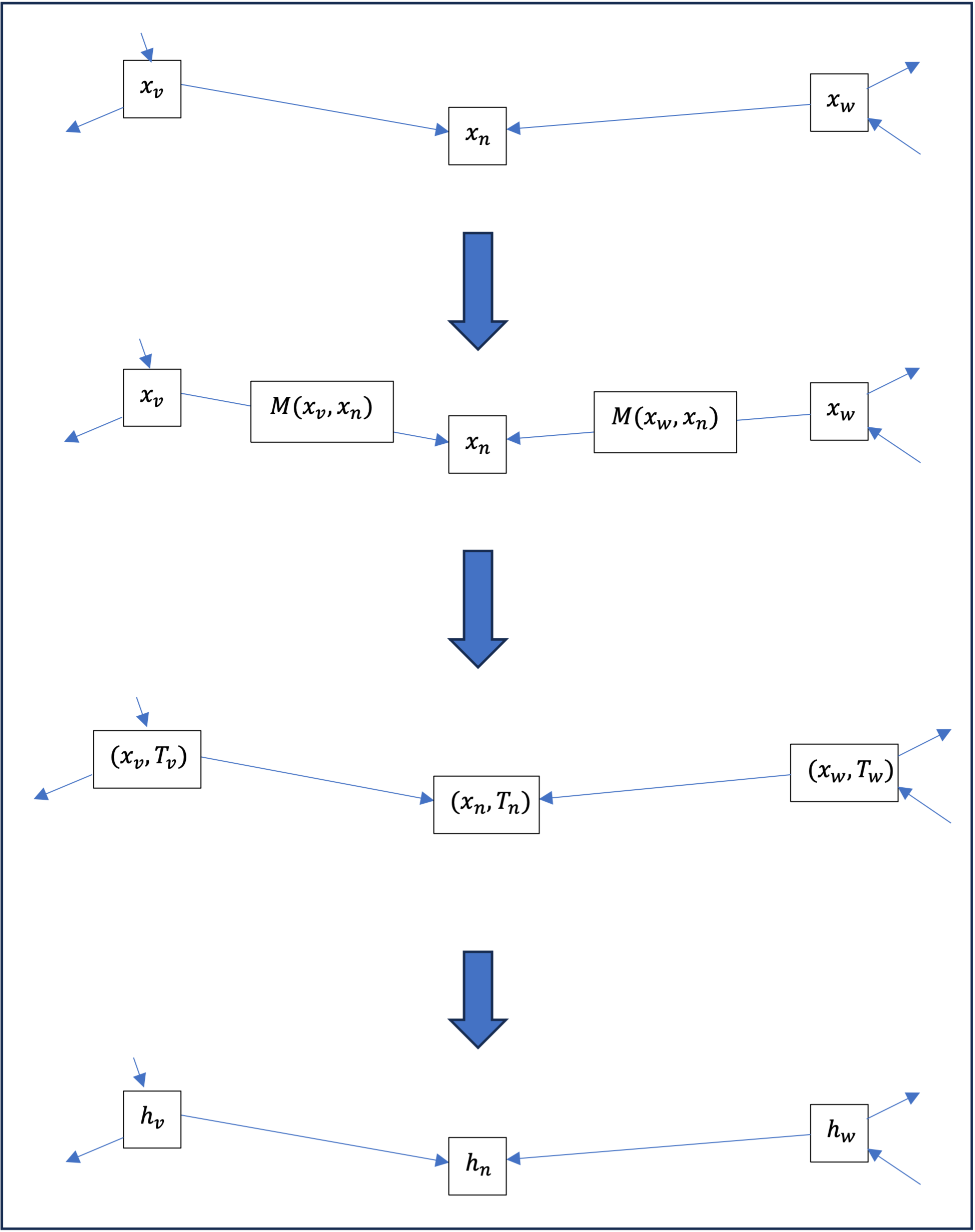
Consider a graph ( G ) and for each node ( n ) , a vector ( x_n in \mathbb{R}^ {m} ) . In the broadest sense, a message transmission layer is a function which for each node \ ( n \ ) will build a new vector ( h_n \in \mathbb{R}^{m'} ) from the vector (x_n\ ) on the one hand, and vectors \ ( x_v\ ) for any node \ ( v\ ) neighbor of \ ( n\ ) as follows :

• For each node \ ( v\ ) neighbor of \ ( n \ ) we calculate the \ ( v\ ) to \ ( n \ ) as a function \ (M \ ) from ( x_n\ ) and ( x_v\ ) :
  \mathrm{Message}_{\{v \to n\}}= M(x_v, x_n).
• All these messages are aggregated into a transmission ( T_n\ ) received by the node ( n \ ) , each individual message being treated on an equal footing; in other words, the aggregation is invariant by permutation of the messages[3]; this is usually done by summing the messages
  T_n = \sum_v M(x_v, x_n),
  or by averaging them out
  T_n = \frac{1}{N} \sum_v M(x_v, x_n),
  Knowing that both sums are taken from the set of neighbors [/] \ ( v\ ) [/] is the size of this set, i.e. the number of neighbors of \ ( n \ ) .
  
• Finally, \ ( h_n\ ) is calculated as a function \ ( P\ ) of the vector \ ( x_n\ ) and the transmission \ ( T_n\ ) :
  h_n = P\!\left(x_n, T_n\right)\!.

Case study: convolution

The typical example of a message transmission layer is the so-called convolution layer[4] where the function \ ( M\ ) returns just the source vector of the message and the aggregation is the sum and the function \ ( P\ ) is an affine function followed by an activation function M\!\left(x,y\right) = x; \\ P\!(x,T) = \sigma\!\left(\!\left(x,T\right)\!A + b\right)\!.

Variations on this message-transmission principle can also be considered, notably in the case where edges are enriched with values that may come into play in the calculation. Another example is the attention layer [5] (or Transformer), where the message is calculated in two stages, the first of which is used to calculate an attention coefficient for each node. \ ( v\ ) neighbor of \ ( n\ ) which is normalized with respect to all its neighbors \alpha\!\left(x_v, x_n\right) = \frac{e^{A\left(x_v, x_n\right)}}{\sum_w e^{A\left(x_w, x_n\right)}}, where \ ( A\ ) is a bilinear function and where the sum is taken over the set of nodes \ ( w\ ) neighbors of \ ( n\ ). We then calculate the message from a neighboring node to the node M\!\left(x,y\right) = \alpha\!\left(x_v, x_n\right)V\!\left(x_v\right) as the product of the attention coefficient and an affine function .

Thus, an example of a method for classifying the nodes of a graph is to successively apply :

1. several layers of message transmission ;
2. then one or more dense layers on each vector associated with a node.

Pooling[6]

The message passing layer (or its variations) is all we need to build graph node classifiers. However, it cannot be used to build classifiers for entire graphs. For this, we can use a layer, or as we shall see, several mutualization layers.

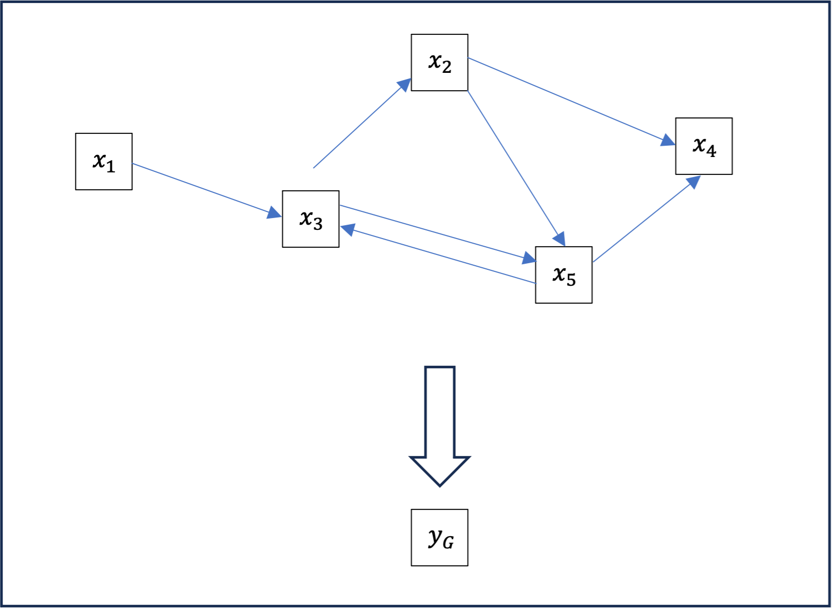
Mutualization is an operation which, starting from a graph where each node is enriched with a vector \ ( x_n \in \mathbb{R}^{m}\ ), produces a new vector \ ( y_G \in \mathbb{R}^{m}\ ) associated with the entire graph. The most commonly used mutualization methods are sum y_G=\sum_n x_n, mean y_G=\frac{1}{N}\sum_n x_n, or maximum y_G=\max_n x_n.

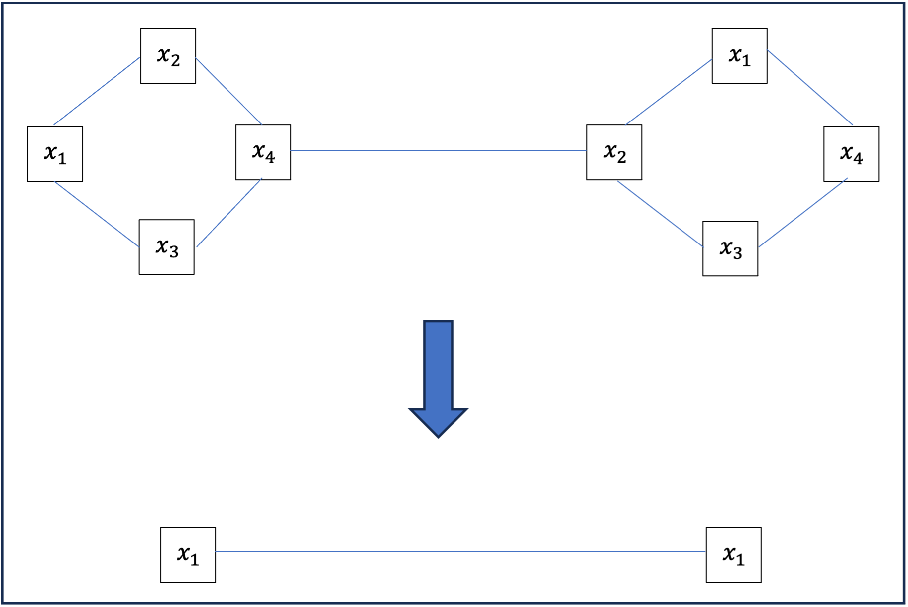
This mutualization operation may seem abrupt; for a large graph, we go from having many vectors and complex relationships between them to a single vector of the same dimension. In many cases, we won’t perform this operation on the complete graph, but on clusters of the graph; we then obtain a new graph whose nodes are clusters of the previous one, as in the following example where y_{1,2,3,4} = \sum_{1}^4 x_i, \ y_{5,6,7,8} = \sum_{5}^8 x_i.

Optimizing graph classification

Thus, an example of a graph classification method is to apply successively on a graph :

1. several layers of message transmission ;
2. pooling by cluster ;
3. again, several layers of message transmission on the cluster graph;
4. global pooling ;
5. finally, one or more dense layers on the shared vector.

This method of calculating and applying graph neural networks is used at Heptalytics to combat fraud and establish fraud & LCBFT scoring.

---

[1] Justin Gilmer, Samuel S. Schoenholz, Patrick F. Riley, Oriol Vinyals, and George E. Dahl. 2017. Neural message passing for Quantum chemistry. In Proceedings of the 34th International Conference on Machine Learning – Volume 70 (ICML’17). JMLR.org, 1263-1272

[2] L. Wu, P. Cui, J. Pei, and L. Zhao. Graph Neural Networks: Foundations, Frontiers, and Applications. Springer, Singapore, 2022, section 4.2.

[3] Euan Ong, Petar Veličković Proceedings of the First Learning on Graphs Conference, PMLR 198:43:1-43:22, 2022.

[4] Kipf TN, Welling M. Semi-supervised classification with graph convolutional networks. In: 5th International Conference on Learning Representations, ICLR 2017, Toulon, France, April 24-26, 2017, Conference Track Proceedings, OpenReview.net

[5] See Veličković, P., Casanova, A., Liò, P., Cucurull, G., Romero, A., & Bengio, Y. (2018). Graph attention networks. OpenReview.net. https://doi.org/10.17863/CAM.48429

[6] L. Wu, P. Cui, J. Pei, and L. Zhao. Graph Neural Networks: Foundations, Frontiers, and Applications. Springer, Singapore, 2022, section 9.3.